GeoSci 236: Gram-Schmidt Orthogonalization

Gidon Eshel
491 Hinds
Dept. of the Geophysical Sciences,
5734 S. Ellis Ave., The Univ. of Chicago,
Chicago, IL 60637
(773) 702-0440, geshel@midway.uchicago.edu

french version

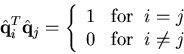
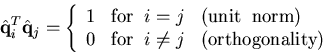
If we have a set of linearly-independent but non-orthogonal vectors ${\bf x}_1$ , ${\bf x}_2\cdots{\bf x}_N$ , we often wish to turn them into an alternative set of vectors, $\hat{\bf q}_1$ , $\hat{\bf q}_2\cdots\hat{\bf q}_N$ , that are mutually orthonormal,

$\begin{displaymath}\hat{\bf q}_i^T\hat{\bf q}_j= \left\{\begin{array}{ll}1&{\rm for}\;\;i=j \\ 0&{\rm for}\;\;i\neq j \end{array}\right.\end{displaymath}$

Achieving this orthonormalization is the purpose of the Gram-Schmidt procedure.

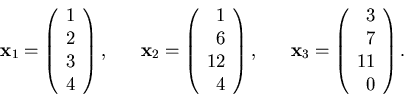
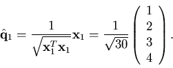
Let's address the particular example of

$\begin{displaymath}{\bf x}_1=\left(\begin{array}{r}1\\ 2\\ 3\\ 4\end{array}\righ... ...bf x}_3=\left(\begin{array}{r}3\\ 7\\ 11\\ 0\end{array}\right).\end{displaymath}$

The first is simple, involving a simple normalization;

$\begin{displaymath}\hat{\bf q}_1=\frac{1}{\sqrt{{\bf x}_1^T{\bf x}_1}}{\bf x}_1=... ...sqrt{30}}\left(\begin{array}{r}1\\ 2\\ 3\\ 4\end{array}\right).\end{displaymath}$

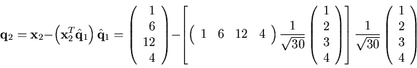
The second vector will be the original second vector, ${\bf x}_2$ , minus its projection on the first orthonormal basis vector, $\hat{\bf q}_1$ . That is,

$\begin{displaymath}{\bf q}_2={\bf x}_2-\left({\bf x}_2^T\hat{\bf q}_1\right)\hat... ...\sqrt{30}}\left(\begin{array}{r}1\\ 2\\ 3\\ 4\end{array}\right)\end{displaymath}$

$\begin{displaymath}{\bf q}_2=\left(\begin{array}{r}1\\ 6\\ 12\\ 4\end{array}\rig... ...}{6}\left(\begin{array}{r}-7\\ 10\\ 33\\ -28\end{array}\right),\end{displaymath}$

which, upon normalization to unit norm, becomes

$\begin{displaymath}\hat{\bf q}_2=\frac{1}{\Vert{\bf q}_1\Vert 6} \left(\begin{ar... ...rray}{r} -0.156 \\ 0.222 \\ 0.734 \\ -0.623 \end{array}\right).\end{displaymath}$

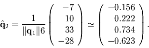
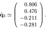
To construct the last basis vector, we need to subtract from ${\bf x}_3$ its projections on both $\hat{\bf q}_1$ and $\hat{\bf q}_2$ ;

$\begin{displaymath}{\bf q}_3 = {\bf x}_3 -\left({\bf x}_3^T\hat{\bf q}_1\right)\hat{\bf q}_1 -\left({\bf x}_3^T\hat{\bf q}_2\right)\hat{\bf q}_2.\end{displaymath}$

Sparing you the straightforward yet tedious arithmetic,

$\begin{displaymath}{\bf q}_3\simeq \left(\begin{array}{r} 2.760 \\ 1.629 \\ -0.724 \\ -0.961 \end{array}\right)\end{displaymath}$

which, when normalized, becomes

$\begin{displaymath}\hat{\bf q}_3\simeq\left(\begin{array}{r} 0.806 \\ 0.476 \\ -0.211 \\ -0.281\end{array}\right).\end{displaymath}$

To test the results, we need to make sure that

$\begin{displaymath}\hat{\bf q}_i^T\hat{\bf q}_j=\left\{\begin{array}{ll} 1&{\rm ... ...\rm for}\;\;i\neq j\;\;\;(\rm orthogonality) \end{array}\right.\end{displaymath}$

as required.

In conclusion, we have transformed our original, non-orthonormal, basis set,

$\begin{displaymath}{\bf x}_1=\left(\begin{array}{r}1\\ 2\\ 3\\ 4\end{array}\righ... ...bf x}_3=\left(\begin{array}{r}3\\ 7\\ 11\\ 0\end{array}\right),\end{displaymath}$

to an entirely equivalent set, whose vectors are all mutually orthogonal and have unit norms. Now, when we express an arbitrary vector from the space spanned by these 2 alternative sets as a linear combination of the orthonormal vectors $\hat{\bf q}_1$ , $\hat{\bf q}_2$ and $\hat{\bf q}_3$ , the projections (the weights) are entirely independent of one another, and their sum is exactly the norm of the represented vector, and not more. This is the reason orthonormalization of the basis vectors is very useful.