Chaotic interpolation

        The reversible transformation of a vector into a pseudo-random or chaotic vector makes it possible to carry out operation of an approximate but fast interpolation.
        The principle of the interpolation is simple:
        We only have to sample the signal with a different number of points from the original sampling and to calculate the new amplitude of each point if this point does not correspond to a sample of the signal origin. Many methods are available which approximate the theoretical interpolation as well as possible.
        Our approach does not aim an algoritmic effectiveness but a demonstration of possibility of processing the signal by methods transposable to the neuromimetic circuits .
        To obtain a number of samples lower than the original one we propose to remove samples of the original signal and this in a uniform random way over all the duration of the signal. The number of points to be removed being proportional to the ratio signal interpolated /original signal.
        We obtain an approximate interpolated signal because of the shift of the samples on the x axis . The problem is to improve the precision of it.
        We thus repeat the operation with a different random sampling which shifts the samples in a different way and we make the average of the obtained interpolated signals .
        It is seen that with successive iterations the sampled points will oscillate around an average value which will be close to the desired value.
        We present below the model matlab which carries out this operation:

Nb_zeros=200; % the original vector comprises 1024 samples, the interpolated vector 1024-200 = 824, ratio=0,80
Iter=200; % Iteration count
Sum_moy_red=zeros(1, size(Cyc_moy, 2)-Nb_zeros); % Initialisation of the vector sum
        for i=1:Iter
                Cyc_bom=bomb_alea(Cyc_moy, Nb_zeros);
                Cyc_moy_red=[Cyc_moy(find(Cyc_bom)), zeros(1, size(Cyc_bom, 2)-Nb_zeros-size(Sum_moy_red, 2)) ]; % suppression of the 0
                                                                                                                                                                                    % and adjustment vector if necessary
                Sum_moy_red=Sum_moy_red+Cyc_moy_red; % Sum reduced vector
        end
Cyc_moy_red=Sum_moy_red/Iter; % Average
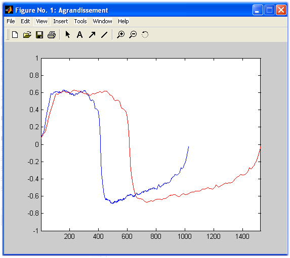
h=figure(1);
set(h,' name',' Origin and Interpolated Cycles',' resize',' off');
axis([1,1024,-1,1 ]);
hold one;
plot(Cyc_moy);
plot(Cyc_moy_red,' color',' r']);

function x=bomb_alea(Cible, Nb_zeros)
% random bombardment of a target vector
% by Nb_zeros

if nargin==0;
       Cible=[1:1:200];Nb_zeros=20; % values of test
end

fin=size(Cible, 2);
vec_01=ones(1, fin);
position=1;
Nb_points=1;
while Nb_points <= Nb_zeros
         position=floor(Rand(1)*(fin-1)+1);
         while vec_01(position)==0
                 position=floor(Rand(1)*(fin-1)+1);
         end
         vec_01(position)=0;
         Nb_points=Nb_points+1;
end
x=Cible.*vec_01;

       In the following program using a chaotic transformation of the vector, only the function bomb_alea changes. It is noticed there that one "cuts" the chaotic vector to the wished length, replacing the part removed by zeros which will be removed by the function find( ) of matlab

function x=bomb_alea2(Cible, Nb_zeros)

if nargin==0; % Values of test
        Cible=[1:1:200 ];
        Nb_zeros=20;
end

fin=length(Cible);
pas_premier=primes(2000); % Primes values list
n=length(pas_premier);
choix=ceil(Rand(1)*n);
pas=pas_premier(choix); % One chooses a step with the hazard in the list of primes values

while rem(fin+1, pas)==0 % if the step is a divider of fin+1 one draws a new step
        choix=ceil(Rand(1)*n); % does not occur if "fin" is even
        pas=pas_premier(choix);
end
for i=1:fin
       position(i)=modulo(i, not, fin+1); % Vector of addresses
       Cible_crypt(position(i))=Cible(i); % Iindexed addressing
end
x_c=[Cible_crypt(1:fin-Nb_zeros), zeros(1, Nb_zeros) ]; % Section of the chaotic vector
x=x_c(position); % Rebuild the vector including Nb _ zeros randomly distributed

       It is noticed that the signal is "less filtered" with a chaotic sampling, which is more regular than a random sampling

We can apply the same principle to enlarge the signal.

It is a question this time of adding samples (Nb_zeros) to the initial signal (Cible). Each sample is the average of the adjacent samples of the initial signal.

function Vect_augm=bomb_alea3(Cible,Nb_zeros)
% chaotic interpolation enlargment
if nargin==0; % default values
    Cible=[1:1:200];
    Nb_zeros=50;
end
fin=size(Cible,2)+Nb_zeros;
vec_01_org=zeros(1,size(Cible,2)+Nb_zeros);
vec_01_org(1:size(Cible,2))=1;
vec_01=zeros(1,size(Cible,2)+Nb_zeros);
Vect_augm=ones(1,fin);
pas_premier=primes(2000);
n=length(pas_premier);
choix=ceil(rand(1)*n);
pas=pas_premier(choix);% One chooses a step with the hazard in the list of primes values
while rem(fin+1,pas)==0 % if the step is a divider of fin+1 one draws a new step
     choix=ceil(rand(1)*n);
     pas=pas_premier(choix);
end
for i=1:fin
     position(i)=modulo(i,pas,fin+1);
     vec_01(position(i))=vec_01_org(i);
end vec_01(1)=1;
vec_01(fin)=1;
curseur=1;
for index=1:fin
     if vec_01(index)~=0
          Vect_augm(index)=Cible(curseur);
          if curseur <= size(Cible,2)-1
               curseur=curseur+1;
          end
     end
     if vec_01(index)==0
           Vect_augm(index)=(Cible(curseur-1)+Cible(curseur))/2;
     end
end
% figure;
% plot(Vect_augm);

Here the result:
Nb_zeros=500; % the vector of origin comprises 1024 samples, the vector interpolated 1024+500=1524, ratio=1.48
Iter=100; % Iteration count

       The principle can of course apply to the processing of an image and thus constitute a pretreatment supplementing the orthogonalisation necessary to maximum storage on an associative memory. In the phase of image recognition , the structure in loop allows moreover the slip of the image by simply modifying the starting point from where the reading begins on the loop.